這段程式碼是使用 R 語言的 ggmap 和 ggforce 函式庫來繪製地圖並在地圖上標註指定位置的周圍半徑範圍內的圓形區域。以下是程式碼的主要步驟:
- 設定 Package、Google Maps API 金鑰: 首先我們載入 ggmap 使用
register_google函數設定 Google Maps API 金鑰,這是為了能夠使用 Google Maps 的地圖服務。而 ggforce 是為了調用 Google Maps 來進行後續的繪圖使用。
library(ggmap)
library(ggforce)

# 設定 Google Maps API 金鑰
register_google(key = apikey)
- 讀取數據: 從指定的 CSV 文件中讀取地名列表,該文件包含站序和站名,需注意的是必須要將格式指定為 UTF-8,否則有時會發生無法正常讀取中文字符串的情況。
station <- read.csv("/Users/hans/Documents/taroko_bus/data/station.csv", encoding = "UTF-8")
- 地理編碼: 使用
geocode函數將地名列表中的站名轉換為地理座標(經度和緯度)。但這邊我們因為無法一次就抓到正確位址所以透過加入關鍵字的方式來輔助 Google Maps 搜尋,同時剔除搜尋錯誤如範圍在台灣之外的結果再重新搜尋一次。
# 要轉換的地名列表
locations <- data.frame(count=station$站序8181[1:38],
                        station=station$站名8181[1:38])
taitung_add <- "taitung, taitung city, taitung county, taiwan 950"
words <- c("", "公車站", "站", "車站", "花蓮", "台東")

location_row <- 1:dim(locations)[1]
geocodeds <- data.frame()
for(word in words){
  geocoded <- geocode(paste0(locations$station, word),
                      output = "more", source = "google")
  geocoded <- cbind(location_row, geocoded)
  if(word=="花蓮"){
    inspace <- which(geocoded$location_row>9)
    geocoded$address[inspace] <- NA
  }else if(word=="台東"){
    geocoded$address[which(geocoded$address==taitung_add)] <- NA
  }
  locations <- locations[which(is.na(geocoded$address)==T |
                               geocoded$lon>=125 | geocoded$lon<=120 |
                               geocoded$lat>=25 | geocoded$lat<=21),]
  geocoded <- geocoded[which(is.na(geocoded$address)==F &
                             geocoded$lon<=125 & geocoded$lon>=120 &
                             geocoded$lat<=25 & geocoded$lat>=21),]
  geocodeds <- rbind(geocodeds, geocoded)
  location_row <- locations$count
}
- 計算圓形坐標點: 根據指定的中心點經緯度和半徑,計算圓形的坐標點。
# 指定中心點經緯度和半徑
center <- data.frame(lon = geocodeds$lon, lat = geocodeds$lat)  # 中心點的經緯度
radius_km <- 1  # 半徑,單位為公里

# 將半徑從公里轉換為度
radius_deg <- radius_km / 111.32  # 每緯度大約111.32公里
- 繪製地圖: 使用
get_map函數取得地圖圖像,然後使用ggmap函數將地圖加載到output中。接著,使用geom_point和geom_path函數在地圖上標註中心點和圓形區域,最後將結果顯示在地圖上。
# 使用 get_map 函數取得地圖圖像
map <- get_map(location = c(center$lon[10], center$lat[10]), zoom = 11)
output <- ggmap(map)

for(i in 1:nrow(geocodeds)){# 計算圓形的坐標點

  circle_points <- data.frame(
    lon = center$lon[i] + radius_deg * cos(seq(0, 2*pi, length.out = 100)),
    lat = center$lat[i] + radius_deg * sin(seq(0, 2*pi, length.out = 100))
  )

  # 繪製地圖
  output <- output +
    geom_point(x = center$lon[i], y = center$lat[i], size = 3, color = 'red') +
    geom_path(data = circle_points, aes(x = lon, y = lat), color = "red", size = 1)

}

output
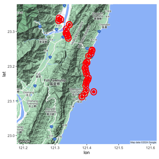
下面是最後顯示在地圖上的結果,紅點為公車站所在的位址,而外圈則為標記半徑一公里的地區。