Question #
我們想要以R語言實作拒絕抽樣的模擬實作,在這裡我們會以蒙地卡羅的方法來將目標函數以覆蓋接受域的作法來實現它。
Method #
首先我們需要給訂一個目標函數 f,同時給定一個生成範圍 [a, b],由於我們想要使用 uniform(0, 1) 來生成符合 f 在 [a, b] 區段機率密度的樣本,因此我們同時需要給定 uniform 的機率密度函數,而α 是一個常數,用於調整拒絕機率,確保生成的樣本符合目標機率密度函數。
對於每個生成的 x 值,計算了對應的機率密度比率 test_x,然後與在 [0, 1] 上生成的隨機數 test_u 進行比較。如果 test_u 小於等於 test_x,則接受該樣本,否則拒絕。
rejection_sampling <- function(f, g, alpha, a, b, n){
  total_n   <- 0
  accept_x  <- c()
  while(length(accept_x) < n){
    total_n <- total_n + 1
    x <- runif(1, a, b)
    test_x <- f(x) / (alpha * g(a, b))
    test_u <- runif(1, 0, 1)
    if (test_u <= test_x){
      accept_x <- c(accept_x, x)
    }
  }
  return(list(c(length(accept_x), total_n), accept_x))
}
Result #
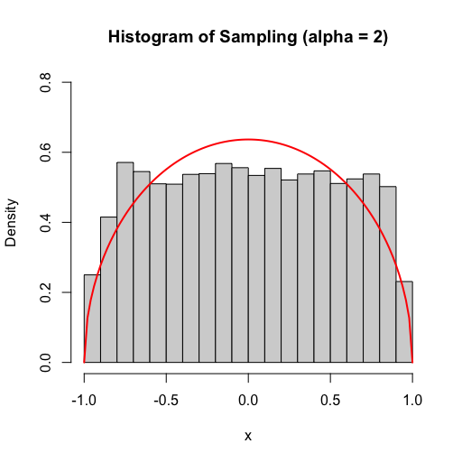
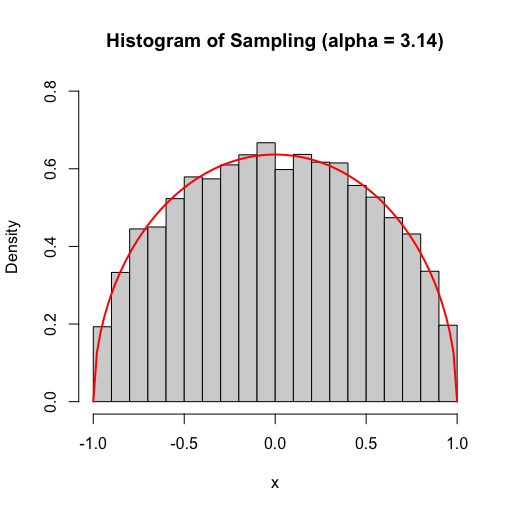
下面我們給定 f 在 [-1, 1]區間,在α = pi的情況下生成 10000 筆模擬資料並繪製結果,紅線是我們的目標函數f,而灰色部分是生成資料的 Histogram。
f <- function(x) pi/2*(sqrt(1-x^2))
unif_pdf <- function(a, b) 1/(b-a)
alpha <- pi
sampling <- rejection_sampling(f, unif_pdf, alpha, -1, 1, 10000)

area <- integrate(f, -1, 1)$value
hist(sampling[[2]], breaks = 15, probability = TRUE,
     xlim = c(-1, 1), ylim = c(0, 0.8), xlab = "x",
     main = paste0("Histogram of Sampling (alpha = " ,round(alpha, 2) ,")"))
curve(f(x) / area, from = -1, to = 1,
      col = "red", lwd = 2, add = TRUE)
Compare α #
最後讓我們來比較在不同 α 的情況下所需迭代次數的變化,可以在下圖中看出在 α = pi 之後所需迭代次數與 α 成正比。
alpha_vector <- c(1, pi/2, pi, 2*pi, 4*pi)
df <- data.frame()
for(alpha in alpha_vector){
  sampling <- rejection_sampling(f, unif_pdf, alpha, -1, 1, 10000)[[1]]
  df <- rbind(df, c(alpha, sampling[2]))
}
colnames(df) <- c("alpha", "iterations")
plot(df$alpha, df$iterations, type = "b", pch = 19, col = "blue",
     xlab = "Alpha", ylab = "Iterations",
     main = "Iterations vs Alpha")
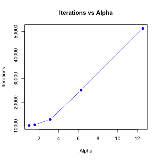
但是在 α < pi 的情況下會導致生成的機率密度無法涵蓋目標函數。這裡的原因是因為計算f(x) / g(a, b)後我們會得到[-0.5, 0.5]這個區間的結果,而函數 f 的最大值為 pi/2,因此如果 α < pi 會導致在函數的最大值部分沒辦法被接受,而因為中央的樣本缺乏導致生成的機率密度較原本而言中間較低兩側較高的情況。